Bike-Sharing Demand Predictor

This is a personal skills showcase, not a client project. It was completed as the capstone for the IBM Applied Data Science with R course on Coursera. It is presented here transparently to demonstrate practical R and data science capability.

The problem

Demand and supply rarely match

Urban bike-sharing systems regularly face a mismatch between bike availability and rider demand. During peak periods, stations run empty; during quiet periods, bikes sit unused. Operators need accurate demand forecasting to redistribute bikes efficiently and reduce both shortages and waste.

The goal of this project was to build a predictive model for hourly bike rental demand using weather and time-of-day data, and to make that model accessible through an interactive dashboard.

Key findings

What drives demand

5×

Seasonal variation in demand

3,556

Peak rentals in a single hour

0°C

Critical usage threshold

82%

Best model accuracy

Temperature dominates

Strong linear correlation with demand across all seasons. Usage drops dramatically below 0°C regardless of time of day.

Commuter-driven peaks

Clear 8am and 6pm usage spikes indicate transport-focused demand. Evening leisure use extends peaks to 10pm in summer.

Rainfall matters most

Rainfall and humidity are the strongest individual predictors — cyclists avoid wet conditions above all else.

Exploratory analysis

Seasonal patterns in the data

Hourly rental counts across 2018 show a clear seasonal pattern — minimal usage in January and February, building to 3,500+ rentals per hour at the summer peak in June–August. The dense clustering of points reflects daily commuter rhythms layered on top of the seasonal trend.

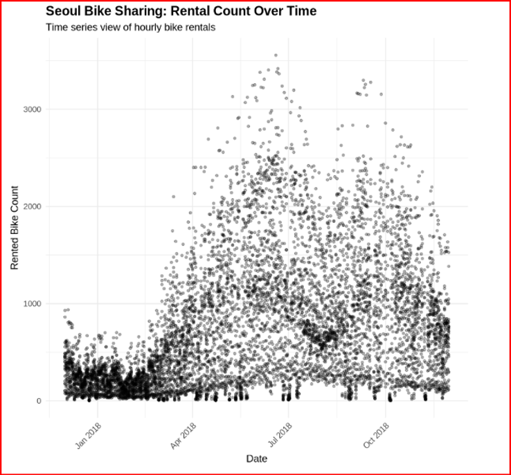
Scatter plot showing Seoul bike rental counts over time throughout 2018, with clear seasonal variation peaking in summer

Seoul Bike Sharing: hourly rental count over time (2018)

Feature importance

Which variables matter

Ranked regression coefficients confirm that rainfall and humidity are the strongest predictors of demand, followed by temperature and specific commuter hours. Wind speed and visibility have minimal effect — cyclists tolerate these conditions but not wet or extreme cold.

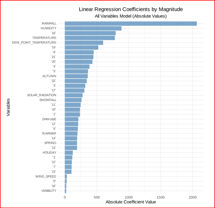
Bar chart showing linear regression coefficients ranked by magnitude, with rainfall and humidity at the top

Linear regression coefficients by magnitude — all variables model

Predictive modelling

Five models compared

Five regression models were developed and evaluated, starting from a baseline linear model and progressively adding polynomial terms, interaction effects, and regularisation. All models exceeded the performance thresholds of R² > 0.72 and RMSE < 330 bikes.

The best performing model — Elastic Net with complex weather interactions — achieved R² = 0.82 and RMSE of 280.8 bikes, successfully capturing the non-linear relationships between weather conditions and demand.

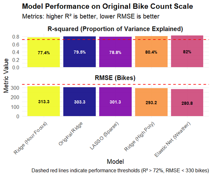
Bar chart comparing R-squared and RMSE across five regression models, with Elastic Net performing best at 82% accuracy

Model performance comparison — R² and RMSE across all five models

Interactive dashboard

Real-time demand forecasting

The project culminates in an R Shiny dashboard that applies the Elastic Net model to generate live demand forecasts for cities worldwide. Users can select a city from the interactive map, view current weather conditions, and explore 5-day temperature and demand prediction trends. The dashboard integrates live data from the OpenWeather API.

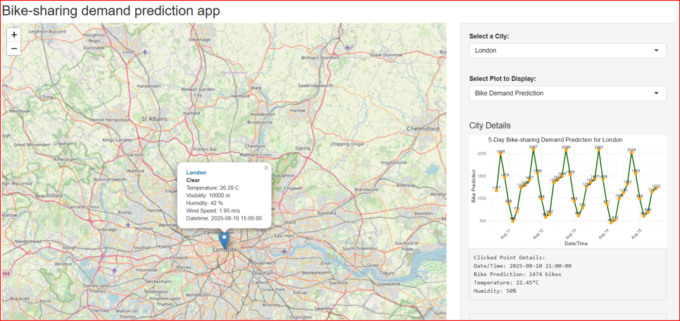
Screenshot of the R Shiny bike-sharing demand prediction dashboard showing an interactive map of New York with weather data and a 5-day temperature trend chart

R Shiny dashboard — city selection, live weather data, and 5-day demand forecast

R / tidyverse R Shiny SQL / SQLite Elastic Net Lasso & Ridge OpenWeather API Web scraping dplyr ggplot2 Leaflet